|
The Bohai Sea is a semienclosed coastal ocean that includes multiple islands and coastal inlets. The mean depth of the Bohai is about 20 m, with the deepest region of about 70 m located near the northern coast of the Bohai Strait. In the Bohai Sea, the motion is dominated by semidiurnal (M2 and S2) and diurnal (K1 and O1) tides, which account for about 60% of the current variation and kinetic energy there. Since the tidally rectified residual flow is only substantial near the coast and islands in the Bohai Sea, geometric fitting is essential to providing a more accurate simulation of the tidal waves and residual flow.
|
|
The Bohai Sea is connected to the Yellow Sea (on the south) through the Bohai Strait. Several islands located in the Strait complicate the water exchange between these two seas. Failing to resolve these islands leads to an underestimation of water transport through the strait. It also results in an unrealistic distribution of the tidal motion in the Bohai Sea due to alterations in the propagation paths of tidal waves. In addition, in the Bohai Sea, the tidally rectified residual flow is usually one order of magnitude smaller than the buoyancy- and wind-induced flows, except near the coast and around islands. In order to obtain a more accurate simulation of temperature and salinity, the model must be able to resolve the complex topography near the coast and around islands.
The Bohai Sea was selected to validate our unstructured grid model (FVCOM) when the model was developed. A comparison was made between structured grid ECOM-si (an updated version of POM) and an unstructured grid FVCOM in the first FVCOM publication written by Chen et al. (2003). Some animations that were made during the validation experiments were selected here to provide a view of tide- and wind-induced circulation in this region. All these animations were made 4-5 years ago. If some one wants to know our updated activities in the Bohai Sea, please contact Dr. Chen at c1chen@umassd.edu.
|
SELECTED MODEL RESULTS and ANIMATIONS
|
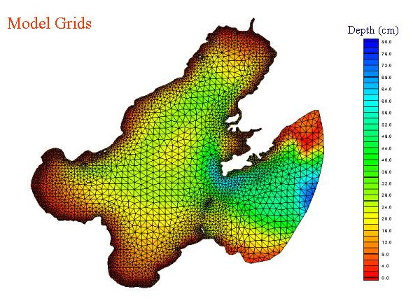
The model domain of FVCOM covers the entire the Bohai Sea, with an open boundary in the Yellow Sea about 150 km south of the Bohai Strait. The horizontal resolution is about 2.6 km around the coast and about 15–20 km in the interior andnear the open boundary. Ten uniformly distributed sigma layers was in the vertical, which result in a vertical resolution of about 0.1–1.0 m in the coastal region shallower than 10 m, and about 6 m at the 60-m isobath. The model were driven using semidiurnal (M2 and S2) and diurnal (O1 and K1) tidal forcing at the open boundary. The initial temperature and salinity were specified using the observed data taken from the one cruise.
|

Click here to view a larger size of this figure. The color is the water depth.
|
An animation showing an example of the near-surface tidal currents in the Bohai Sea. To give a view of the surface elevation, we stretched the vertical coordinate scale when the movie was made. Since this stretch was made inconsistently with the tidal surface elevation, so it caused mismatching between the model surface and bathymetry around the coast. It should be in caution when this animation is used for the tidal elevation. That was the first animation we made by using Open Window DX. No correction was made, because we have already shifted to use ViSiT or Datatank for making animation. ViSiT is the parallelized visualization software that can be used for linux, units, PC and Mac.
|

Click here or images to view a large-size flash movie. |
An animation showing an example of the surface wind used to drive the model. This wind field was downloaded from the reanalaysis result of the weather forecast model for the Pacific Ocean. The wind data were interpolated to the center point of individual triangle. Because of the limitation in horizontal resolution of the wind field, the meso-scale structure of the wind field did not show in this movie. To get the Bohai and Yellow Seas modeling correctly, a need is to upgrade the meso-scale weather forecast system in this region, with at least of 3 km resolution.
We are setting up a WRF for Bohai and Yellow Seas.
Click here or image on the right to view the full-size animation. |

|
 |
|
 |
Model-predicted surface temperature and salinity aimiation for a stratified case with the only tidal forcing.
Click here or image above to watch a bigger size of animation.
|
Model-precited surface temperature and salinity aimiation for the case with tides and surface heat flux.
Click here or image above to watch a bigger size of animation.
|
Model-predicted surfce temperature and salinity aimiation for the case with tidal and wind forcing plus heat flux.
Click here or image above to watch a bigger size of animation.
|
Case 1:
Particle trajectories for a homongeous case with the only tidal forcing. Red balls: particles released near the surface; Blue balls: particles released at the local middle depth.
Click here or image above to watch a bigger size of animation. |
 |
Case 2:
Particle trajectories for a stratified case with tidal forcing. Water temperature and salinity at initial were specified by the observed data. Particles were released at the same level as shown in case 1.
Click here or image above to watch a bigger size of animation. |
|
Case 3:
Particle trajectories for a stratified case with tidal and wind forcing. Initial conditions for water temperature and salinity were the same as those in case 2.
Click here or image above to watch a bigger size of animation. |
|
Case 4:
Particle trajectories for a stratified case with tidal and wind forcing plus surface heat flux. Initial conditions for water temperatur and salinitity were the same as those in cases 2 and 3.
Click here or image above to watch a bigger size of animation. |
|
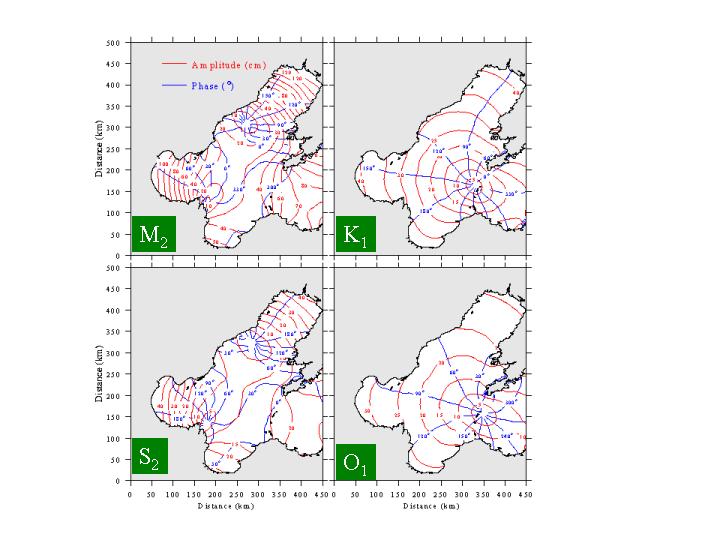
Model-Predicted Co-tidal Charts
FVCOM shows that M2 and S2 tidal waves propagate counterclockwise around the coast like a Kelvin wave.
The model predicts two nodes of the M2 and S2 tides in the Bohai Sea: one is near the mouth of the Yellow River on the southwestern coast, and the other is located offshore of Qinhuangdao on the northwestern coast. These two nodes. The maximum amplitudes of the M2 and S2 tides are about 130 cm in Liaodong Bay and 100 cm in Bohai Bay. FVCOM shows similar structures for the K1 and O1 tides. The comparison between observed and model-predicted tidal elevation at measurement stations were given in Chen et al. (2003).
Click here or image to view a full-size of figure.
|

|
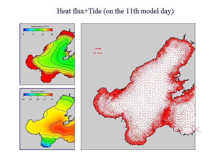
Stratified Residual Currents
For the stratified case initialized with the hydrographic field measurement data, the model driven by tides and surface heat flux predicted a cyclonic near-coastal residual current around the Bohai Sea plus complex circulation around islands. Failure to resolve islands near the Bohai Strait, which was often the case in previous finite-different structured grid modes, can cause an overestimation of the cross-strait water transport and destroy the round-coastal currents near the Bohai Strait.
Click here or image to view a full-size of figure.
|

|
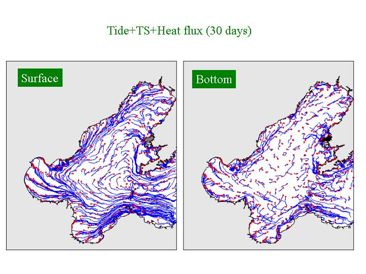
Particle Trajectories
Trajectories of particles for a period of 30 days for the case with tides plus surface heat flux. Red dots: the locations where particles were released. This figure shows clearly a round-coastal cyclonic circulation pattern near the surface.
Click here or image to view a full-size of figure.
|

|
Results of A Simple NPZ Coupled Physical-Biological Model |
|
Case 1: Only Tidal Forcing
The initial conditions of water temperture and salinity were specified using the field measurement data. The biological values at initial were given by vertical profiles of NPZ that were uniform everywhere in the horizontal. In the case, the model was driven only by tidal forcing.
Click here or image to watch animation.
|
 |
Case 2: Tidal and Wind Forcing
The model setup in this case was the same as case 1 except adding the wind forcing. The objective of this experiment was to see how NPZ fields responded to the wind-driven circulation and mixing.
Click here or image to watch animation.
|
 |
Case 3: Tidal and WInd Forcing plus Heat Flux
The model setup in this case was the same as case 2 except adding surface heat flux. The objective of this experiment was to see how NPZ fields responded to the variability of the surface heat flux.
Click here or image to watch animation.
|
 |
|