|
 |
 |
|
Tidal Simulation |
The observed sea elevations at the 7 along-estuary stations (green dots on site map of right) from Julian day 23 through 72 in 1999 during the GARLMER 8 observational period was processed and calibrated by Dr. Blanton.
Harmonic analyses were used to construct amplitudes and phases of five major tidal constituents (M2, S2, N2, K1 and O1) of water level at these 7 sites. The harmonic analysis method is based on Foreman's (1977) tidal height harmonic analysis program, which provides tidal amplitudes and phases and their standard deviations with a 95% confidence level.
Click here or image to view larger image.
|
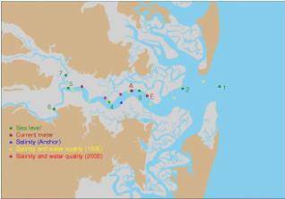 |
Fig.1. The Satilla River Estuary (the observation sites of tide and salinity are shown in different legends)
|
|
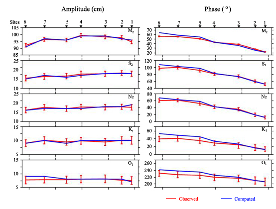
The FVCOM hydrodynamic model was driven by M2, S2, N2, K1 and O1 tidal elevations and phases at the open boundary. The model was run for tidal simulation over 40 days and then model-output water levels were processed using the harmonic analysis program. |

Fig.2 Comparison between model-predicted (blue line) and observed (red line) amplitudes and phases of M2, S2, N2, K1 and O1 tidal constituents. The red bars indicate the uncertainty range of tidal measurement. Click here or image to view larger image. |
The comparison results show that the model has provided a reasonably accurate simulation of the amplitudes and phases of semi-diurnal (M2, S2, and N2) and diurnal (K1 and O1). The red error bars are sample standard deviations at a 95% confidence level. All the model-predicted amplitudes are within uncertainty level of field measurement. The difference of phases between model-predicted and observed are less than 15o at upstream, and most of them were within uncertainty level of the measurement.
|
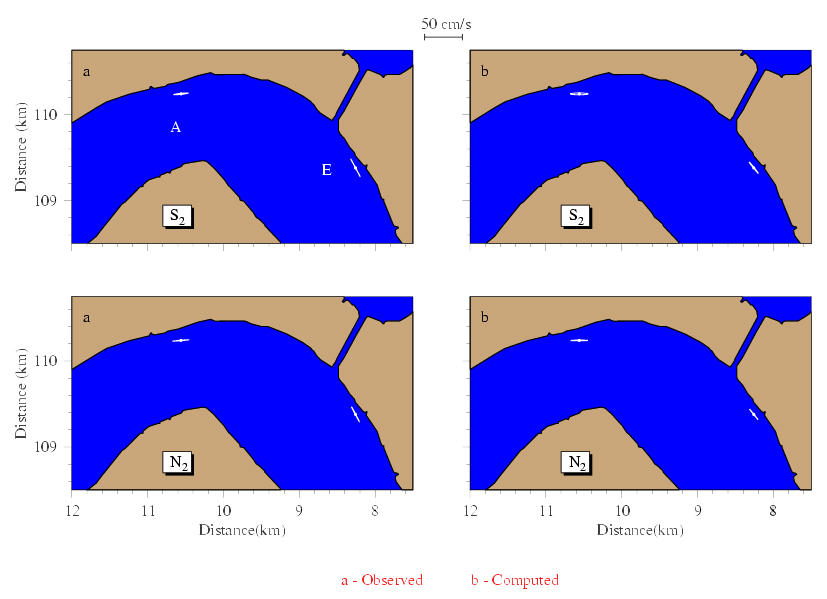
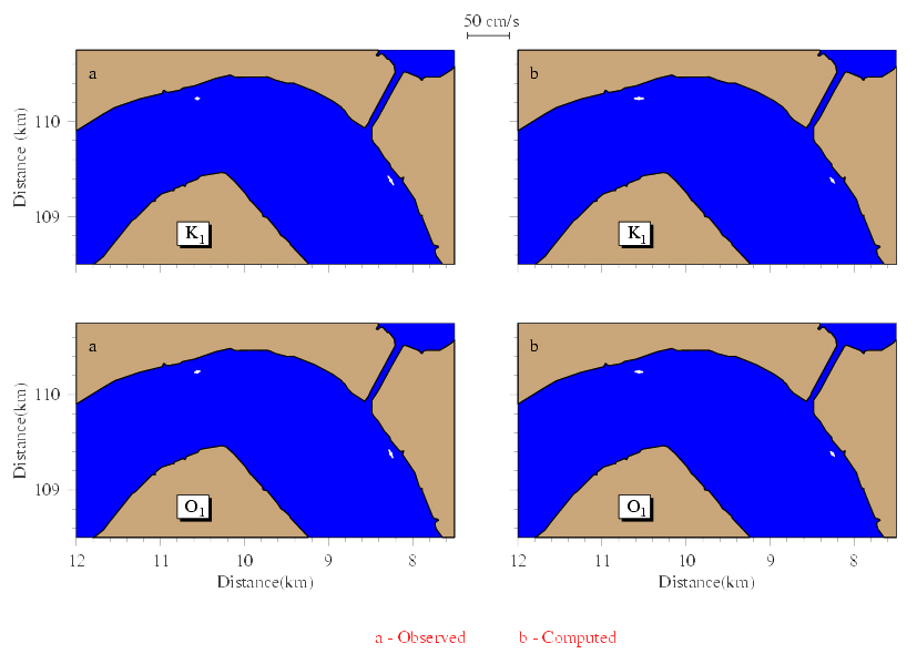
The stations A and E for the observed current velocity are shown in site map (red rectangles). The data was also from Dr. Jack Blanton at Skidaway Institute of Oceanography. The model-predicted tidal current elliptic parameters of the M2, S2, N2, K1 and O1 tidal constituents were in good agreement with those of observations.
Numerical experiments were also carried out to examine the importance of the inclusion of the intertidal salt marsh in the tidal simulation. The comparison of the results for the cases with and without the inclusion of the flooding/drying process shows that the intertidal salt marsh is a key geometric reason that remains the large water transport into the estuaries. Ignoring the intertidal salt marsh results in a significant underestimation of the tidal current up to 50%. This suggests that in order to get the physics correct, the estuarine hydrographic model must include the water movement over the salt marsh.
Fig.3 Comparison between observed (up) and model-predicted (low) M2 tidal current ellipses at two current meter-mooring sites (in Fig. 1 A and E). Click here or image to view a larger image.
|
|
|
Fig.4. Comparison between observed (left) and model-predicted (right) S2 and N2 tidal current ellipses at two current meter-mooring sites. Click here or image to view larger image. |
Fig.5. Comparison between observed (left) and model-predicted (right) K1 and O1 tidal current ellipses at two current meter-mooring sites. Click here or image to view larger image. |
|
|
|
|
Contact:
Dr. Changsheng Chen
School for Marine Science
and Technology
University of Massachusetts Dartmouth
email: c1chen@umassd.edu
Dr. Mac V. Rawson
Georgia Sea Grant College Program
University of Georgia
Athens, GA 30602
email: mrawson@uga.edu
Dr. Randal L. Walker
Marine Extension Service
University of Georgia
Athens, GA 30602-3636
email: walker@uga.edu
|
|
Copyright ©
2005
SMAST/ UMASSD
All rights
reserved | |
|
 |
|